Overview
Teaching: 0 min Exercises: 0 minQuestions
What machine learning techniques are available in GEE?
How do I perform supervised classification of satellite imagery?
How do I assess the accuracy of my classifier?
How do I create my own geometries manually?
Objectives
Practice finding cloud-free imagery and using hand-drawn geometry imports
Learn the basic functions necessary to train and apply a classification algorithm
Evaluate training accuracy using a confusion matrix
Classifiers Overview
Google Earth Engine provides users with the opportunity to conduct many advanced analysis, including spectral un-mixing, object-based methods, eigen analysis and linear modeling. Machine learning techniques for supervised and unsupervised classification are also available. In this example, we will use supervised classification for land cover classification.
The purpose is to get a classified map of land cover in an area of interest. We will examine Landsat imagery and manually identify a set of training points for three classes (water, forest, urban). We will then use those training points to train a classifier. The classifier will be used to classify the rest of the Landsat image into those three categories. We can then assess the accuracy of our classification using classifier.confusionMatrix().
Link to full code we used in this session: https://code.earthengine.google.com/c6c3d195c2d2b00d8852f0ac0cd1ef99
Adapted from the Earth Engine 201 Intermediate workshop
Exercise: Creating a land cover classification from Landsat imagery
Creating an ROI from coordinates
First we need to define a region of interest (ROI). Instead of using an imported asset, we will use a single coordinate that we will manually define. I am interested in doing a classification around Houston, so I will use the city center as my lat/long.
// Define a region of interest as a point.  Change the coordinates
// to select an ROI in your area of interest.
// You can use the inspector tool to find your coordinates
var roi = ee.Geometry.Point(-95.6223, 29.7381);
Loading an ImageCollection and filtering to a single image
Now we will load Landsat imagery and filter to the area and dates of interest. We can use sort to filter the ImageCollection by % cloud cover, a property included with the Landsat Top of Atmosphere (TOA) collection. We then select the first (least cloudy) Image from the sorted ImageCollection .
// Load the Landsat 8 scaled radiance image collection.
var landsatCollection = ee.ImageCollection('LANDSAT/LC08/C01/T1')
    .filterDate('2017-01-01', '2017-12-31');

// Make a cloud-free composite.
var composite = ee.Algorithms.Landsat.simpleComposite({
  collection: landsatCollection,
  asFloat: true
});

// Visualize the Composite
Map.addLayer(composite, {bands: ['B4', 'B3', 'B2'], max: 0.5, gamma: 2}, 'L8 Image', false);
Collect Training Data
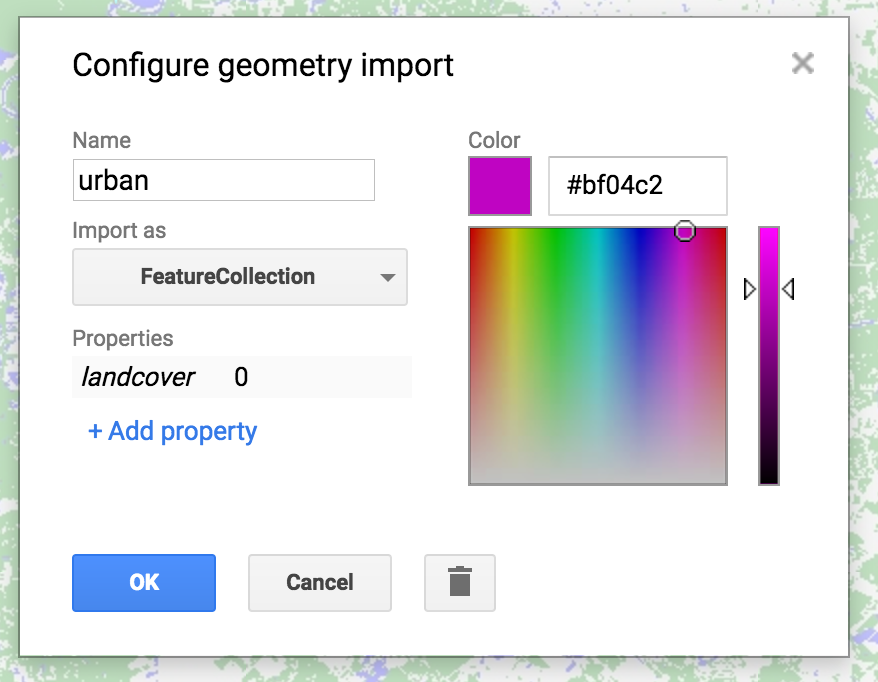
The second step is to collect training data. Using the imagery as guidance, hover over the ‘Geometry Imports’ box next to the geometry drawing tools and click ‘+ new layer.’ Each new layer represents one class within the training data. Let the first new layer represent ‘urban.’ Locate points in the new layer in urban or built up areas (buildings, roads, parking lots, etc.). When finished collecting points, click ‘Exit’ and configure the import (top of the script) as follows. Name the layer ‘urban’ and click the icon to configure it. ‘Import as’ FeatureCollection. ‘Add property’ landcover and set its value to 0. (Subsequent classes will be 1 for water, 2 for forest, etc.) when finished, click ‘OK’ as shown:
When you are finished making a FeatureCollection for each class (3 total), you now can merge them into one FeatureCollection using featureCollection.merge(). This will convert them into one collection in which the property landcover has a value that is the class (0, 1, 2).
// Merge points together
var newfc = water.merge(urban).merge(forest);
print(newfc, 'newfc')
The print statement will display the new collection in the Console.
Sample Imagery at Training Points to Create Training datasets
Now that you have created the points and labels, you need to sample the Landsat 8 imagery using image.sampleRegions(). This command will extract the reflectance in the designated bands for each of the points you have created. A conceptual diagram of this is shown in the image below. We will use reflectance from the optical, NIR, and SWIR bands (B2 - B7).

// Select the bands for training
var bands = ['B2', 'B3', 'B4', 'B5', 'B6', 'B7'];

// Sample the input imagery to get a FeatureCollection of training data.
var training = composite.select(bands).sampleRegions({
  collection: newfc,
  properties: ['landcover'],
  scale: 30
});
The FeatureCollection called training has the reflectance value from each band stored for every training point along with its class label.
Train the classifier
We will now instantiate a classifier using ee.Classifier.randomForest() and train it on the training data specifying the features to use (training), the landcover categories as the classProperty we want to categorize the imagery into, and the reflectance in B2 - B7 of the Landsat imagery as the inputProperties.
// Make a Random Forest classifier and train it.
var classifier = ee.Classifier.randomForest().train({
  features: training,
  classProperty: 'landcover',
  inputProperties: bands
});
Other classifiers, including Support Vector Machines (SVM) and Classification and Regression Trees (CART) are available in Earth Engine. See the Supervised Classification User Guide for more examples.
Classify the Image & Display the Results
Use the new classifier to classify the rest of the imagery.
// Classify the input imagery.
var classified = composite.select(bands).classify(classifier);
// Define a palette for the Land Use classification.
var palette = [
'D3D3D3', // urban (0) // grey
'0000FF', // water (1) // blue
'008000' // forest (2) // green
];
// Display the classification result and the input image.
Map.setCenter(-96.0171, 29.6803);
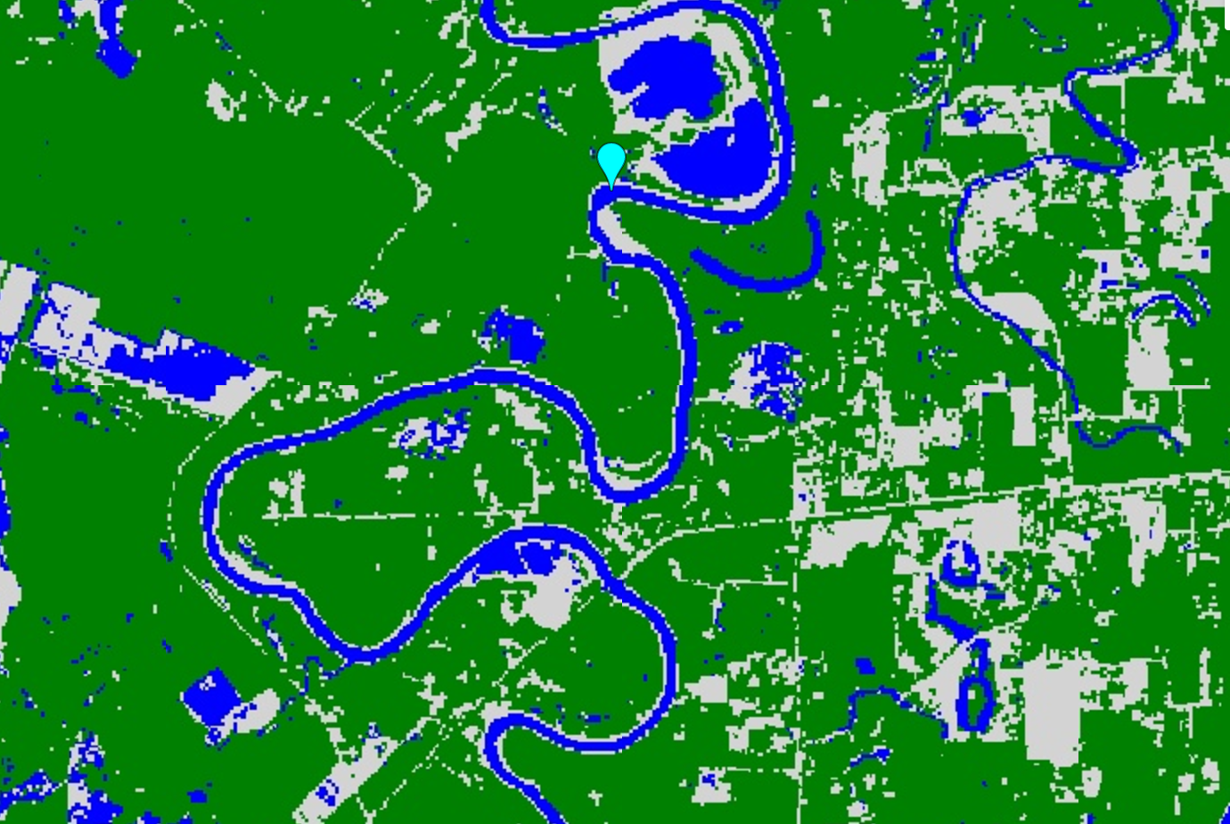
Map.addLayer(classified, {min: 0, max: 2, palette: palette}, 'Land Use Classification');You should get an image that looks sort of like the one below. Pan around the map and use the inspector to and see how you did!
Assess the Accuracy
We can assess the accuracy of the trained classifier using a confusionMatrix.
// Get a confusion matrix representing resubstitution accuracy.
print('RF error matrix: ', classifier.confusionMatrix());
print('RF accuracy: ', classifier.confusionMatrix().accuracy());
Word of warning: In this particular example, we are just looking at the trainAccuracy, which basically describes how well the classifier was able to correctly label resubstituted training data, i.e. data the classifier had already seen. To get a true validation accurcay, we need to show the classifier new ‘testing’ data. The repository code has a bonus section at the end that holds out data for testing, applies the classifier to the testing data and assesses the errorMatrix for this withheld validation data. The last example in the Supervised Classification User Guide also gives example code for this process.
Key Points
GEE can be used for both supervised and unsupervised image classification.
The general workflow for classification includes gathering training data, creating a classifier, training the classifier, classifying the image, and then estimate error with an independent validation dataset.
Confusion matrices can be used to assess the accuracy of supervised classifiers but should be used with caution.